Numpy

NumPy is a package for scientific computing that allows calculation algebraic manipulation of matrices with n dimensions.

To import NumPy in your Python code:

1
import numpy as np

In the NumPy website, there is a tutorial that explains how to start.

The basic data type is ndarray which represents a multidimensional array. Examples:

1
2
scores = np.array([7.8, 9.1, 8.6, 7.4])
houses = np.array([104, 515, 1], [140, 635, 1], [50, 210, 0])

Linear Algebra

Vector

Vectors can be understood as points in space, and we can represent the data using vectors. E.g. the data that represents a house, student test scores, values that make up the price of a product, etc, can be stored in a vector.

In Python, we represent the vector using an array of NumPy, so if we have only the information of square meters of the house, we have a vector with one axis:

1
house = np.array([67])

Adding the house value, we have a vector with two axes:

1
house = np.array([67, 250])

If we keep adding more house details like the number of bedrooms, we have a vector with three axes:

1
house = np.array([67, 250, 2])

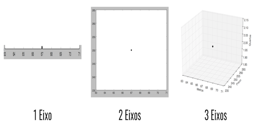
And we keep adding more house details to the vector and at each value, we have a new axis.

Figure 1 shows a vector that can be visually represented until three axes.

Figure 1: Visualizing a vector with 1, 2, and 3 axes.

Useful methods to work with np.array

1
2
3
4
x = np.array([1, 2, 3, 4])
x.sum() # sum the values of the vector = 10
x.min() # min value of the vector = 1
x.max() # max value of the vector = 4

Sum of vectors

Two or more vectors (with the same length) can be summed through the sum of each element in the same position, e.g: when we have a vector with the value of products and another vector with taxes, we can sum both vectors to know how much you spend at each purchased product.

1
2
3
products = np.array([5, 6, 7, 8])
taxes = np.array([1, 2, 3, 4])
sum = products + taxes  #[6, 8, 10, 12]

Scalar sum

In a vector we can sum one value with all elements, this is a scalar sum. E.g. imagine an array of students test score, and we want add 0.5 for each value:

1
2
tests = np.array([6.5, 8.0, 7.5, 4.5, 9.0, 6.5, 6.0, 5.5, 7.0, 8.0, 6.5, 7.5])
tests += 0.5  #[7.0, 8.5, 8.0, 5.0, 9.5, 7.0, 6.5, 6.0, 7.5, 8.5, 7.0, 8.0]

Operations with NumPy’s array

Using tests vector from the previous example, we would like to know how many students have a score test greater or than 7.0. For this, we can apply a comparison in each element:

1
2
3
4
pass = tests >= 7.0
# the result is a boolean vector: 
# array([True, True, True, False, True, True, False, False, True, True, True, True], dtype=bool) 
# True indicates a score greater or equal to 7.0, and False indicates scores less than 7.0.

We can count the True values:

1
amountPass = sum(tests >= 7.0)  #9

The same can be done with students that have the score less than 7.0 and fail:

1
2
fails = tests < 7.0
# array([False, False, False, True, False, False, True, True, False, False, False, False], dtype=bool)

And count how many values are True, that have a score less than 7,0:

1
amountFail = sum(tests < 7.0)  # 3

Multiplication of vectors

Two or more vectors can be multiplied. We need multiply each value of the same positions of the vectors:

1
2
3
x = np.array([1, 2, 3, 4])
y = np.array([5, 6, 7, 8])
mult = x * y  #[5, 12, 21, 32]

If we have a vector with scores test from one student:

1
scores = np.array([8.0, 7.0, 7.5, 9.5, 10.0])

And a vector with weight of each test, used to calculate the final score:

1
weights = np.array([0.2, 0.1, 0.1, 0.3, 0.3])

If multiply both vectors and sum all values, we have the student final score:

1
finalScore = sum(scores * weights)

Scalar multiplication

We can multiply a vector by a scalar, so we have a value that will be multiplied by each element of the vector. E.g. suppose that we have a vector of purchased products:

1
products = np.array([18.0, 16.5, 17.0, 19.5, 18.5])

And we want calculate 10% of taxes for each value:

1
taxes = valores * 0.1  #[1.8, 1.65, 1.7, 1.95, 1.85]

If you want to know the sum of all taxes we can sum the vector values sum(taxes).

Scalar product of vectors

Figure 2 shows a scalar product of two vectors.

Figure 2: Equation from the scalar product of two vectors.

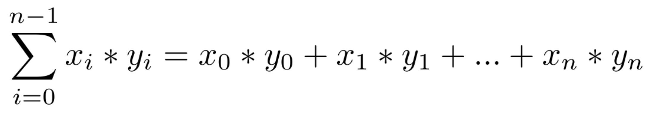
Where x and y are two vectors from same length, and n the length of vectors, the scalar product is the sum of both vectors multiplied:

1
2
3
x = np.array([1, 2, 3, 4])
y = np.array([5, 6, 7, 8])
prod = np.dot(x, y)  # 70

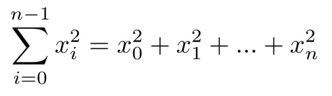
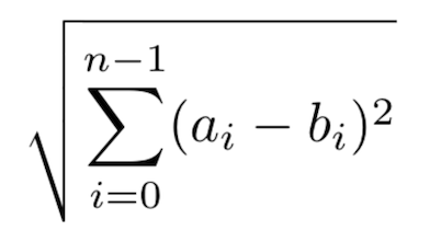
To calculate the sum of squares of a vector, we can use the scalar product, like showing in Figure 3.

Figure 3: Sum of squares of a vector.

1
2
x = np.array([1, 2, 3, 4])
prod = np.dot(x, x)  # 30

The result will be the sum of the multiplication of x vector by itself.

Distance between vectors

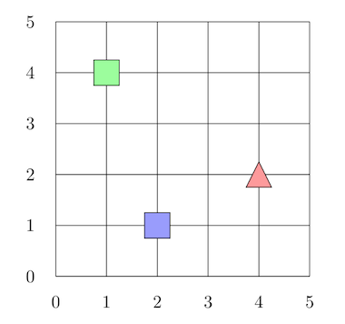
In Figure 4, we have the vector [1,4] (green square) and the vector [2,1] (blue square). If we add a new vector [4,2] (red triangle), but we would like to classify this new vector, as the green or blue vector using the vector distance of other vectors. What is the square closest to the red triangle?

Figure 4: Distance between vectors.

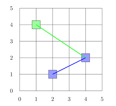
In Figure 5, we can see that the blue square is closest to the red triangle, so we can use this measure to classify the red triangle as being a blue square.

Figure 5: Distance between vectors.

One flavor to calculate the distance between vectors is using the Euclidean Distance, the equation is shown in Figure 6.

Figure 6: Euclidean Distance.

In Figure 7, we calculate the euclidean distance between the vector [1,4] (green square) with the vector [4,2] (red triangle).

Figure 7: Euclidean Distance between green square and red triangle.

In Figure 8, we calculate the Euclidean distance between the vector [2,1] (blue square) with the vector [4,2] (red triangle).

Figure 8: Euclidean distance between blue square and red triangle.

So, now we know that the shortest distance is in relation to the blue square.

Using Python, we can calculate the distance between vectors:

1
2
3
gs = np.array([1,4])    # Green square
bs = np.array([2,1])    # Blue square
rt = np.array([4,2])    # Red triangle

With:

1
2
distanceFromGreenSquare = np.sqrt(sum((qv - tv) ** 2)) #3.6055
distanceFromBlueSquare  = np.sqrt(sum((qa - tv) ** 2)) #2.2360

The ** is used to calculate the left number raised to the right number. Sample: 5² is calculated with 5 ** 2.

Matrixes

Matrix is a set of vectors, normally represented with a capital letter, like A[m, n] that have m lines by n columns. The NumPy has the matrix object that represents a matrix, example:

1
2
A = np.matrix([[1, 2, 3, 4],
               [5, 6, 7, 8]])

In this example, we say that the matrix A has size [2, 4], or two lines and four columns. To access a specific matrix position, we need to inform the value of line and column, remember that the index starts with zero, the value of position A[1, 3] é 8.

Sum of matrices

Sum of matrices:

1
2
3
4
5
6
7
8
A = np.matrix([[1, 2, 3, 4], 
               [5, 6, 7, 8]])
B = np.matrix([[1, 2, 3, 4], 
               [5, 6, 7, 8]])

SUM = A + B
# [[ 2,  4,  6,  8],
#  [10, 12, 14, 16]]

Transposed

Using Numpy we can easily get transposed from a matrix:

1
2
3
4
5
6
A = np.matrix([[1, 2, 3, 4], 
               [5, 6, 7, 8]])
A.T    # [[1, 5],
       #  [2, 6],
       #  [3, 7],
       #  [4, 8]]

Matrix multiplication

When we multiply two matrices, the matrix A has the dimension m x n, and matrix B has the dimension n x m, then with the result, we have a matrix with dimension m x m.

1
2
3
4
5
6
7
8
A = np.matrix([[1, 2, 3, 4], 
               [5, 6, 7, 8]])
B = np.matrix([[1, 2],
               [3, 4], 
               [5, 6],
               [7, 8]])
mult = A * B  # [[ 50,  60],
              # [114, 140]]